Visualizations

panchi includes a built-in visualization system for vectors, linear transformations, and vector spaces. Two-dimensional visualizations are accessed through Animator2D, and three-dimensional ones through Animator3D — the two classes share the same five-method API, differing only in dimension. This page documents Animator2D first, then covers what changes in Animator3D.

Setup

panchi ships with a matplotlib backend by default. For higher-quality, video-based output, install the optional manim backend:

pip install panchi[manim]

Creating an animator

from panchi import Vector, Matrix, VectorSpace
from panchi.visualizations import Animator2D

# Interactive display (matplotlib pops up a window)
animator = Animator2D()

# Save to disk instead
animator = Animator2D(save_path="./my_plots")

# Use manim for video output
animator = Animator2D(backend="manim", save_path="./videos")

The backend parameter selects which rendering engine to use. Manim is only imported when you request it, so matplotlib users never need it installed.

Constructor options

Parameter	Default	Description
backend	"matplotlib"	"matplotlib" or "manim"
save_path	None	Directory for output files. If None, matplotlib shows interactively.
quality	"medium"	Render quality: "low", "medium", "high", "production" (manim only)
figsize	(8, 8)	Figure size in inches (matplotlib only)

When save_path is set, static plots are saved as .png and animations as .gif (matplotlib) or .mp4 (manim).

---

Plotting vectors

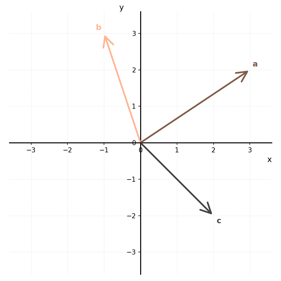
v1 = Vector([3, 2])
v2 = Vector([-1, 3])
v3 = Vector([2, -1])

animator.plot_vectors([v1, v2, v3], labels=["v1", "v2", "v3"])

Pass any number of 2D vectors as positional arguments. Optional parameters:

• colors — list of hex color strings (e.g. ["#FF0000", "#0000FF"])
• labels — list of label strings
• grid — show coordinate grid (default True)
• name — output filename when saving (default "plot_vectors")

Example output.

---

Animating vector addition

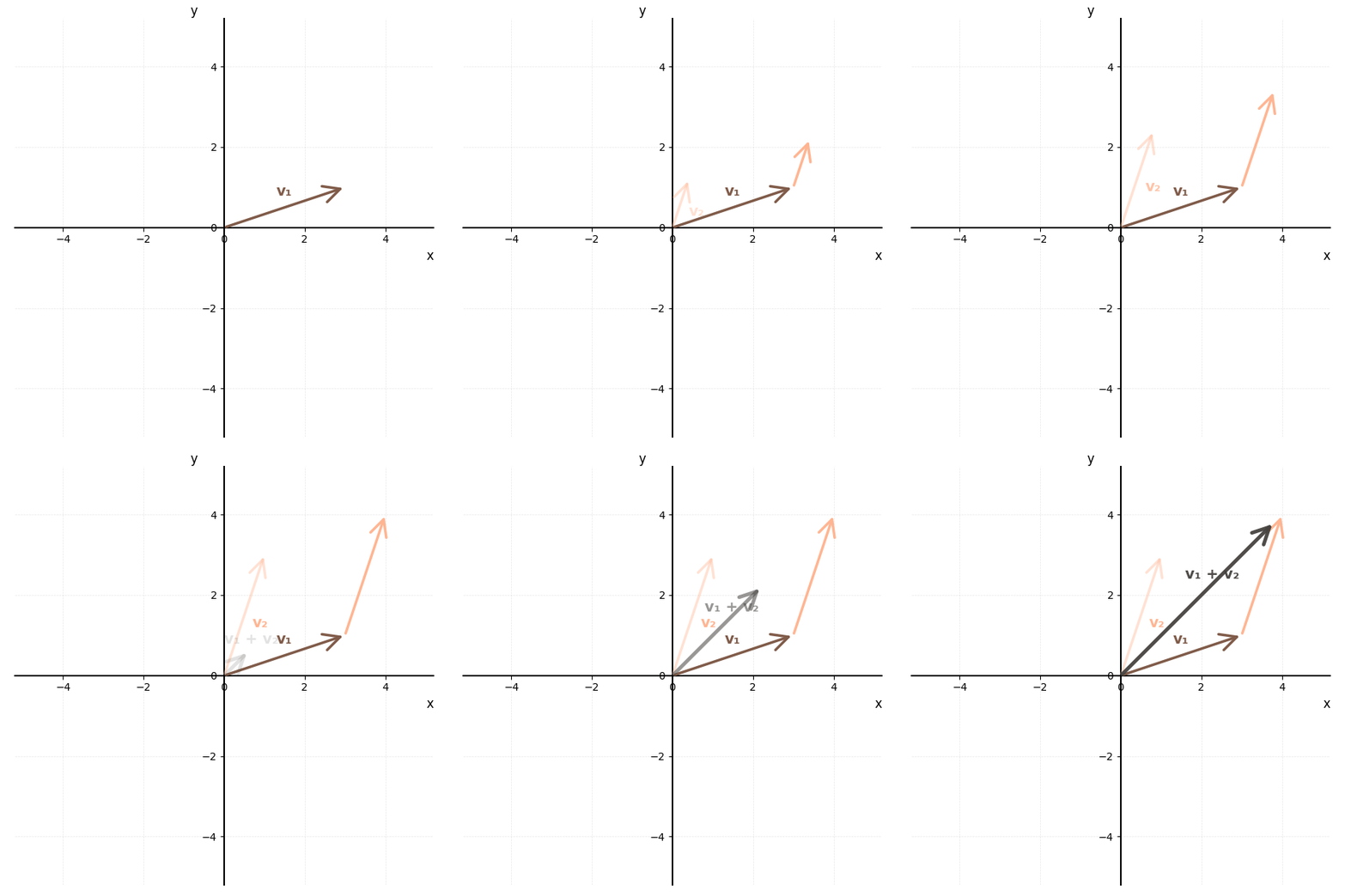
v1 = Vector([3, 1])
v2 = Vector([1, 3])

animator.animate_addition(v1, v2)

The animation shows v1 drawn first, then v2 growing from the origin and from v1's tip simultaneously, and finally the result vector appearing. The manim backend also draws the parallelogram with dashed lines.

Optional parameters: frames, interval (milliseconds between frames), name, and colors (up to three, for [v1, v2, v1 + v2]).

Example output.

---

Animating scalar multiplication

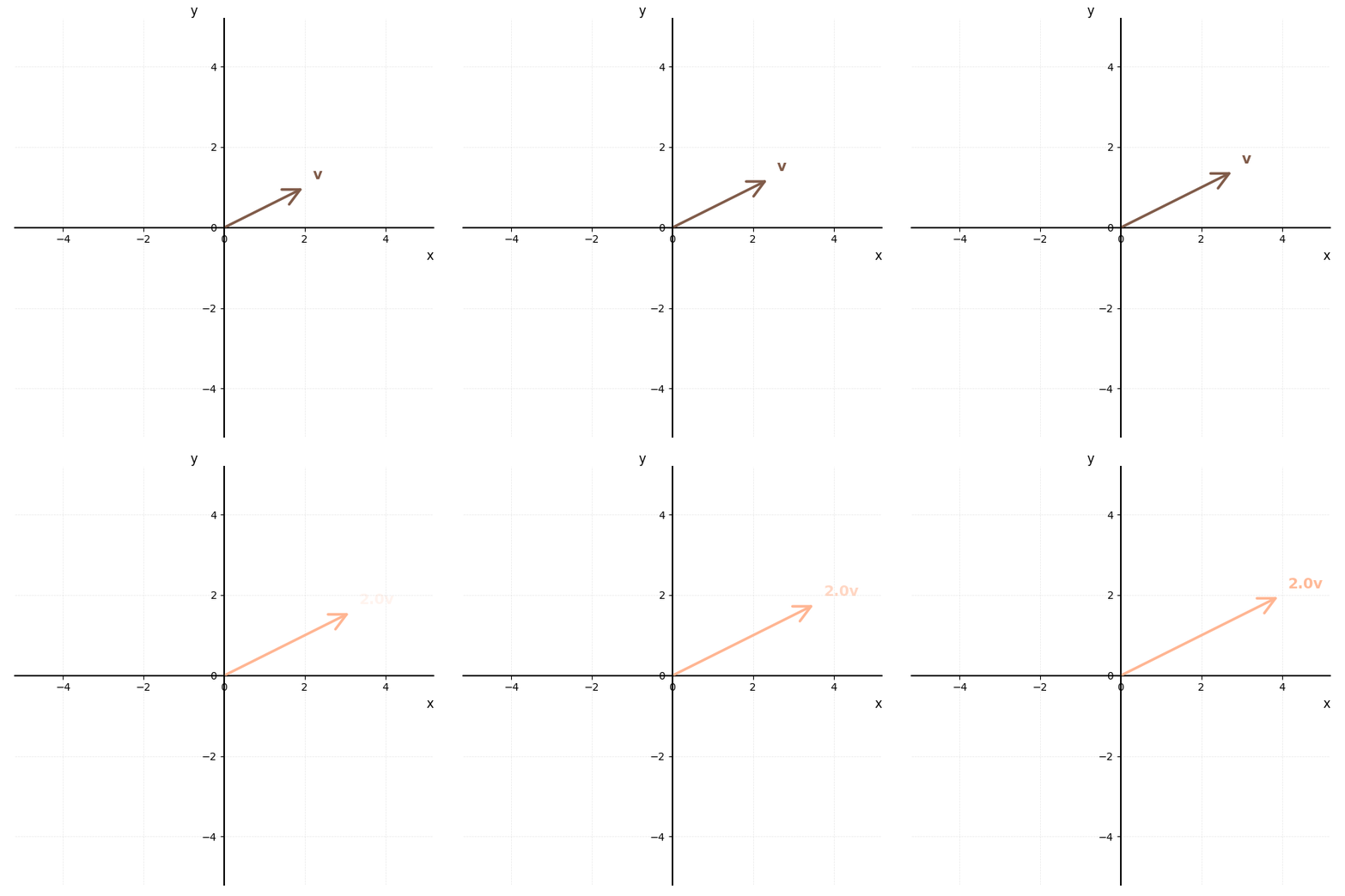
v = Vector([2, 1])

animator.animate_scaling(v, scale_factor=2.5)

The vector smoothly stretches (or shrinks, or flips for negative factors) from its original length to the scaled length.

Optional parameters: frames, interval, name, and colors (up to two, for [original, scaled]).

Example output.

---

Animating linear transformations

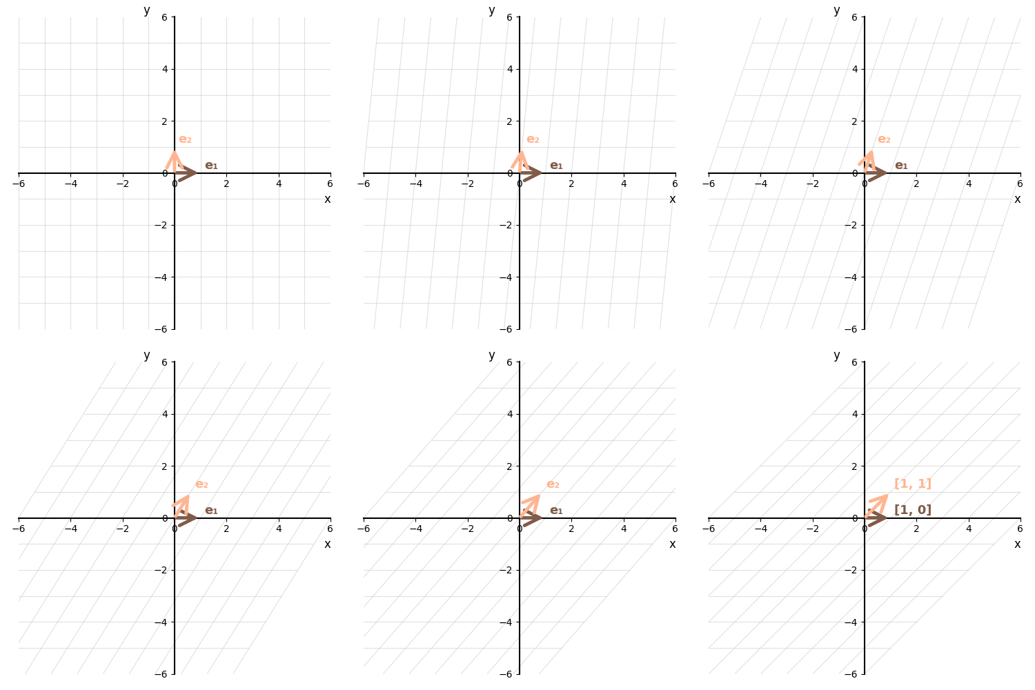
This is the signature visualization — a full grid deformation showing how a 2x2 matrix transforms the plane, in the style of 3Blue1Brown's Essence of Linear Algebra.

# 90-degree rotation
animator.animate_transform(Matrix([[0, -1], [1, 0]]))

# Horizontal shear
animator.animate_transform(Matrix([[1, 1], [0, 1]]))

# Projection onto the x-axis
animator.animate_transform(Matrix([[1, 0], [0, 0]]))

The animation shows:

1. The standard basis vectors e1 and e2 on a coordinate grid
2. The entire grid smoothly morphing from the identity to the target transformation
3. Labels updating to show each vector's coordinates after the transformation

By default the standard basis is transformed. Pass vectors to watch your own vectors slide from v to matrix @ v — useful for seeing where a specific vector lands:

animator.animate_transform(
    Matrix([[2, 1], [0, 1]]),
    vectors=[Vector([1, 0]), Vector([1, 2]), Vector([-1, 1])],
)

Only 2x2 matrices are supported — a ValueError is raised for other shapes.

Optional parameters: vectors, frames, interval, name, and colors (one per transformed vector, cycling if fewer are supplied).

Example output — a horizontal shear.

---

Visualizing spans

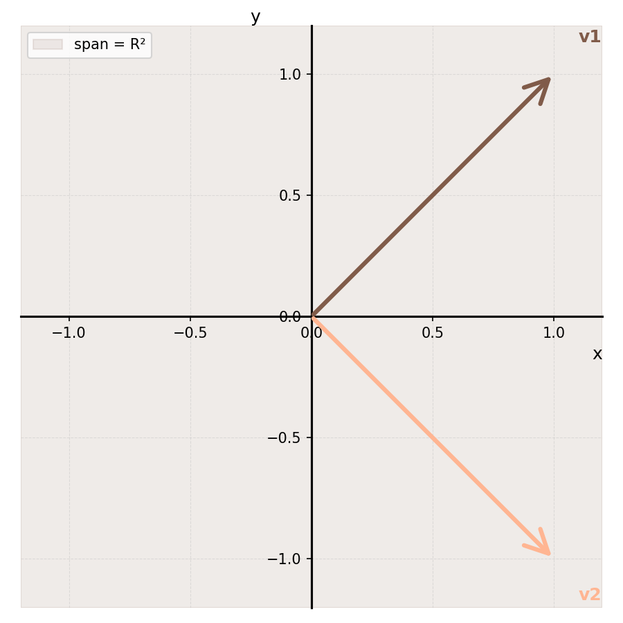
plot_span draws the subspace spanned by a set of vectors, with a shaded region and basis vector arrows.

# From a list of vectors
animator.plot_span([Vector([1, 2])])                      # 1D span (line)
animator.plot_span([Vector([1, 0]), Vector([0, 1])])      # 2D span (full plane)

# From a VectorSpace object
space = VectorSpace([Vector([1, 1]), Vector([1, -1])])
animator.plot_span(space, labels=["v1", "v2"])

The visualization adapts to the dimension of the subspace:

• dim 1 — a line through the origin in the basis direction, highlighted with a colored band
• dim 2 — the entire visible plane shaded to indicate it spans all of R²

If you pass linearly dependent vectors, panchi computes the actual basis automatically:

# These two vectors are parallel — the span is still 1D
animator.plot_span([Vector([1, 2]), Vector([2, 4])])

Example output — two independent vectors spanning R².

Comparing several spans

Pass a list of spans — each a list of vectors or a VectorSpace — to draw them together, each in its own color with a legend. This makes relationships between subspaces visible, such as two distinct lines or a plane against an axis:

animator.plot_span(
    [
        [Vector([1, 1])],              # one line
        [Vector([1, -1])],            # a different line
        VectorSpace([Vector([2, 1])]),  # a third, from a VectorSpace
    ],
    labels=["A", "B", "C"],
)

With multiple spans, colors gives one color per span and labels names them in the legend; span_color applies to the single-span case only.

Optional parameters: colors, labels, grid, name, and span_color (the shade of the span region, single span only).

---

Saving output

When save_path is set, every method saves its output to that directory:

animator = Animator2D(save_path="./output")

animator.plot_vectors([Vector([1, 2])], name="my_vectors")
# → ./output/my_vectors.png

animator.animate_transform(Matrix([[0, -1], [1, 0]]), name="rotation")
# → ./output/rotation.gif  (matplotlib)
# → ./output/rotation.mp4  (manim)

The name parameter controls the filename (without extension). If omitted, it defaults to the method name (e.g. "plot_vectors", "animate_transform").

---

Backend comparison

Feature	matplotlib	manim
Install	Included with panchi	pip install panchi[manim] + system deps
Output format	.png / .gif	.mp4 video
Interactive display	Yes (plt.show())	No (always renders to file)
Grid morph quality	Good (LineCollection interpolation)	Excellent (native NumberPlane)
LaTeX labels	No	Yes
Parallelogram in addition	No	Yes
Render speed	Fast	Slower (video encoding)

Both backends support all five visualization methods with the same API, for both Animator2D and Animator3D.

---

3D visualizations (Animator3D)

Animator3D mirrors Animator2D for vectors in R³. It exposes the same five methods — plot_vectors, animate_addition, animate_scaling, animate_transform, and plot_span — with identical signatures. Everything above about backends, save_path, output formats, and the name parameter applies unchanged; only the geometry becomes three-dimensional.

from panchi import Vector, Matrix, VectorSpace
from panchi.visualizations import Animator3D

animator = Animator3D()                          # interactive matplotlib
animator = Animator3D(save_path="./output")      # save .png / .gif
animator = Animator3D(backend="manim", save_path="./videos")

The constructor takes the same parameters as Animator2D (backend, save_path, quality, figsize). The only difference: for 3D the quality tiers are "low", "medium", and "high" — there is no "production" tier.

All vectors passed to Animator3D must be 3D; a 2D vector raises a ValueError.

Plotting vectors

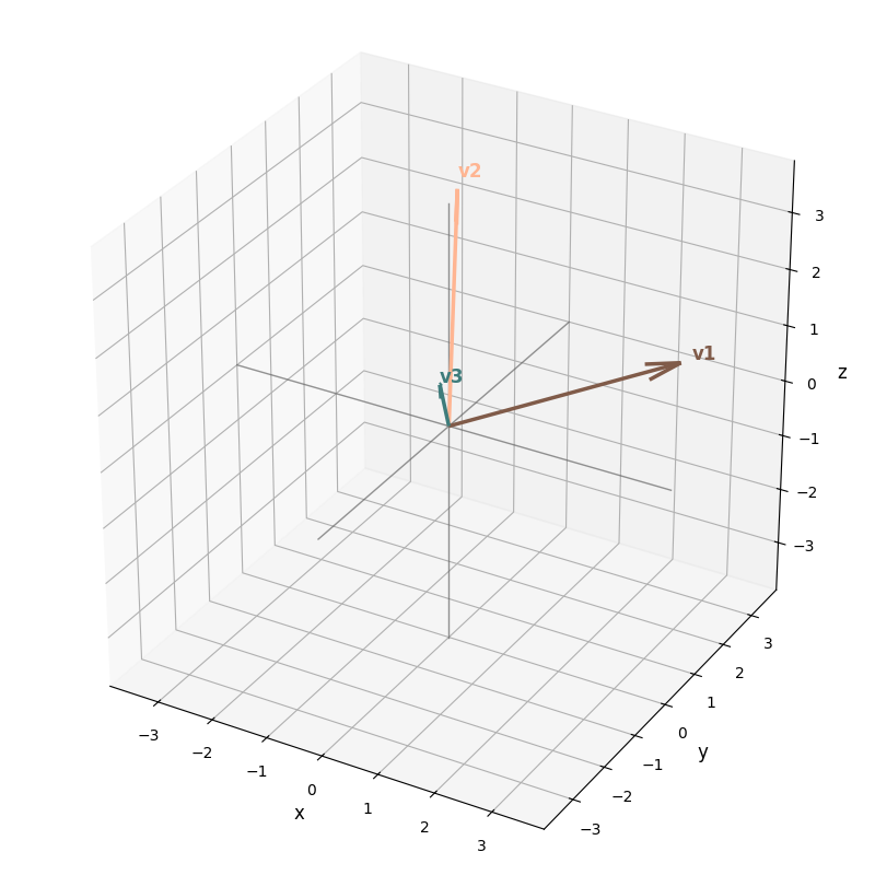
animator.plot_vectors(
    [Vector([3, 2, 1]), Vector([-1, 2, 3]), Vector([1, -2, 2])],
    labels=["v1", "v2", "v3"],
)

Each vector is drawn as a 3D arrow from the origin inside an x/y/z coordinate box. Accepts the same colors, labels, grid, and name options as the 2D version.

Example output.

Animating vector addition

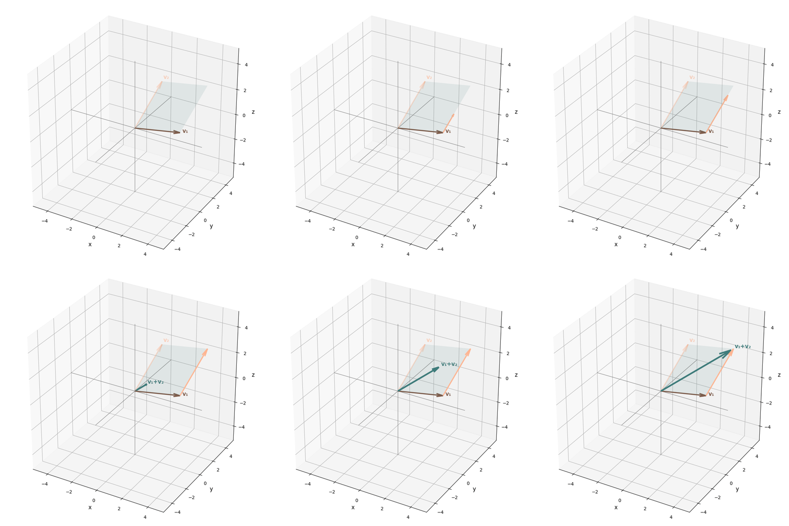
animator.animate_addition(Vector([3, 1, 0]), Vector([1, 2, 3]))

Draws v1, then v2 growing tip-to-tail from v1, and finally the result — with the parallelogram spanned by v1 and v2 shown as a translucent face. Same frames, interval, name, and colors ([v1, v2, v1 + v2]) options as in 2D.

Example output.

Animating scalar multiplication

animator.animate_scaling(Vector([2, 1, 1]), scale_factor=2.0)

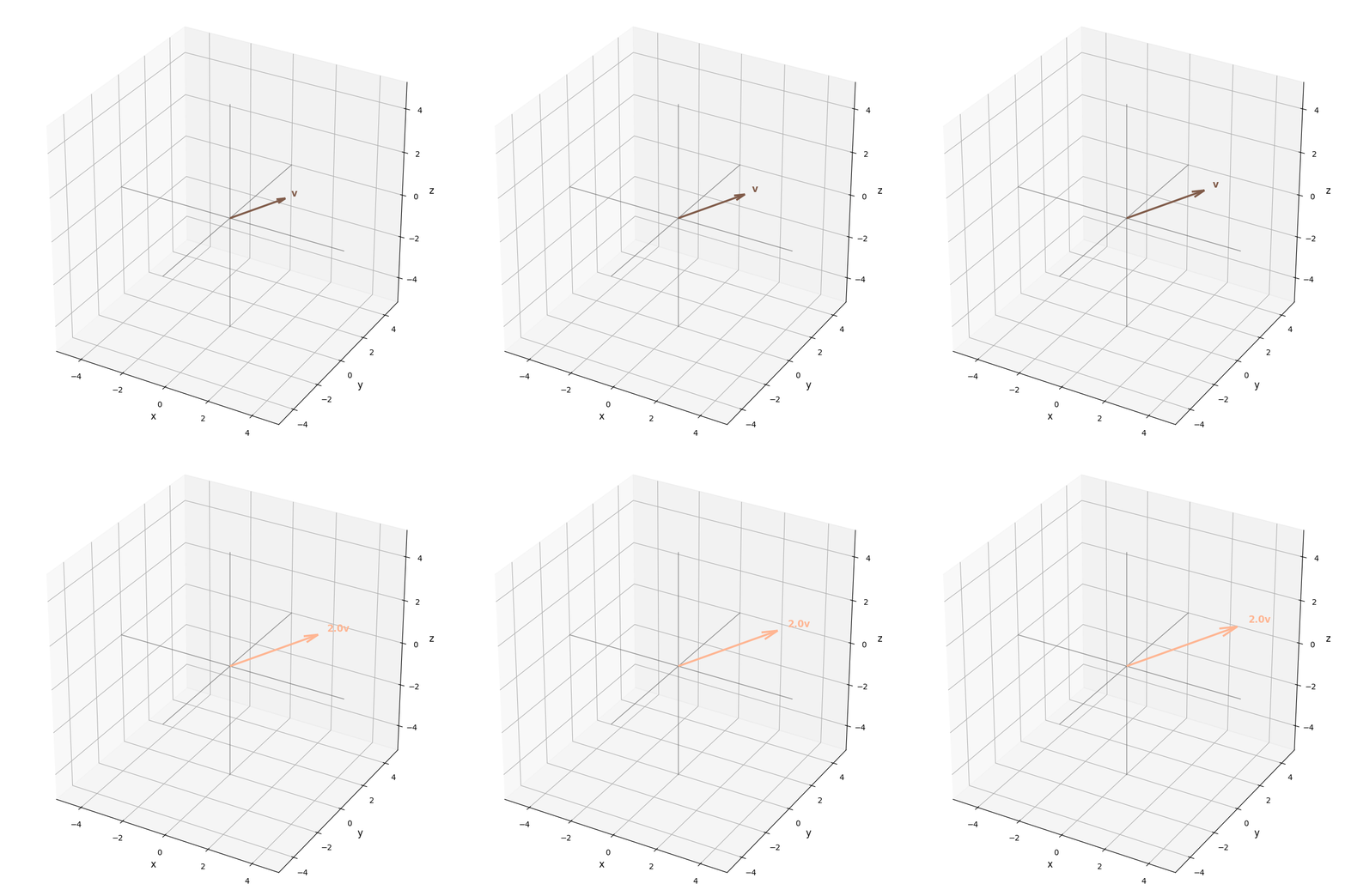
The vector stretches, shrinks, or flips in R³ exactly as in the 2D case. Options: frames, interval, name, and colors ([original, scaled]).

Example output.

Animating linear transformations

# rotate 45° about the z-axis
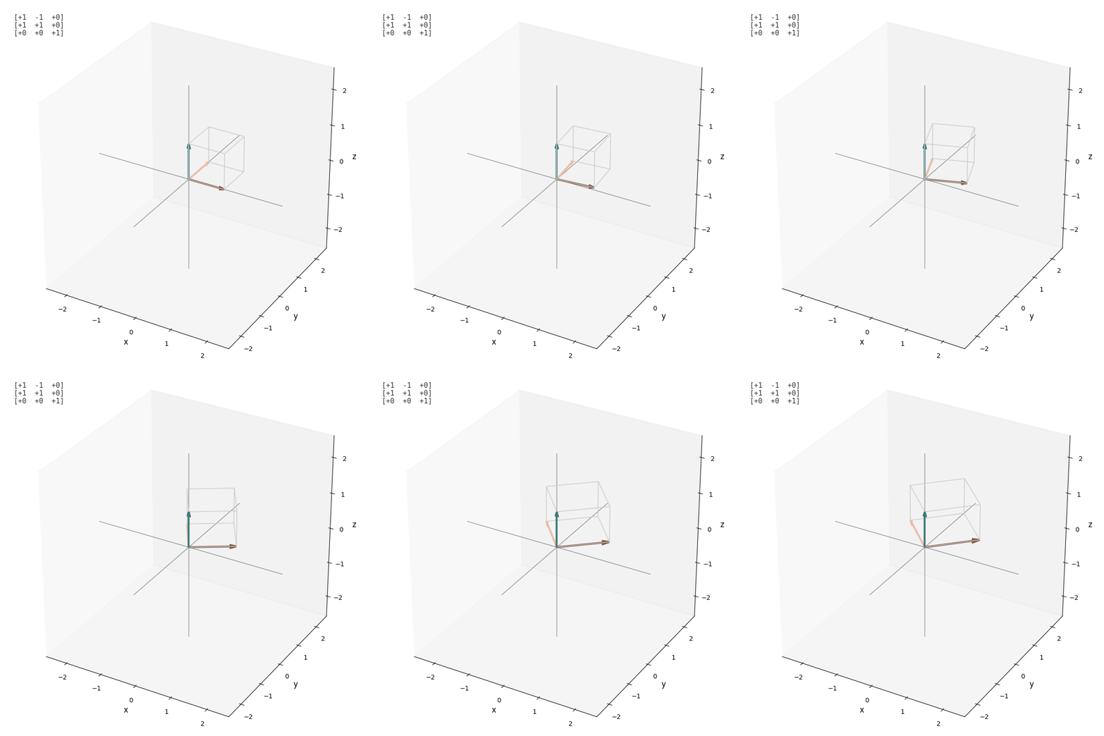
animator.animate_transform(Matrix([[1, -1, 0], [1, 1, 0], [0, 0, 1]]))

The 3D analogue: each vector slides from v to matrix @ v, with the matrix shown as an overlay. By default the three standard basis vectors are transformed (their images are the columns of the matrix). Pass vectors to transform your own instead:

animator.animate_transform(
    Matrix([[2, 0, 0], [0, 1, 0], [0, 1, 1]]),
    vectors=[Vector([1, 1, 0]), Vector([0, 1, 2])],
)

Only 3x3 matrices are supported — a ValueError is raised for other shapes. Options: vectors, frames, interval, name, and colors (one per transformed vector, cycling if fewer are supplied).

Example output — a rotation about the z-axis.

Visualizing spans

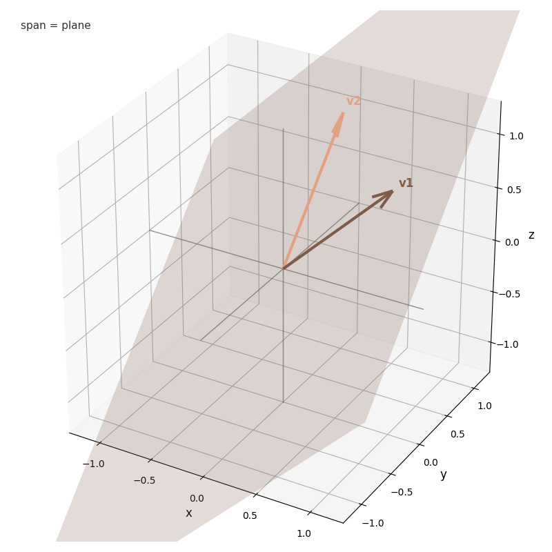
animator.plot_span([Vector([1, 0, 1]), Vector([0, 1, 1])], labels=["v1", "v2"])

plot_span adapts to the dimension of the subspace:

• dim 1 — a line through the origin in the basis direction
• dim 2 — a shaded plane patch through the origin
• dim 3 — a translucent cube indicating the span fills all of R³

As in 2D, linearly dependent vectors are reduced to the true basis automatically, so the drawn dimension reflects the real span. You can also pass a list of spans to compare several subspaces at once — each drawn in its own color with a legend (e.g. a plane against an axis):

animator.plot_span(
    [
        [Vector([1, 0, 0]), Vector([0, 1, 0])],  # the xy-plane
        VectorSpace([Vector([0, 0, 1])]),         # the z-axis
    ],
    labels=["plane", "axis"],
)

Options: colors, labels, grid, name, and span_color.

Example output — two independent vectors spanning a plane in R³.